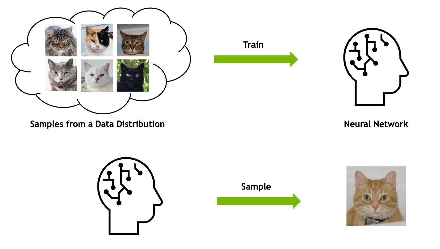
$\color{blue}{\text{Generative Models }}$ 
- Training Dataset : $\{x^{(1)}, \cdots,x^{(N)}\} \sim q_{data}(x)$ ($\color{red}{\text{Do we have this distribution?}}$)
- The main goal is $\rightarrow$ learn a generative model: $P_{\theta}(x)$ such that
- $P_{\theta}(x) \approx q_{data}(x)$ (Realistic Data) (Easy generation)
$\color{blue}{\text{Discriminative Model v.s. Generative Model }}$ 

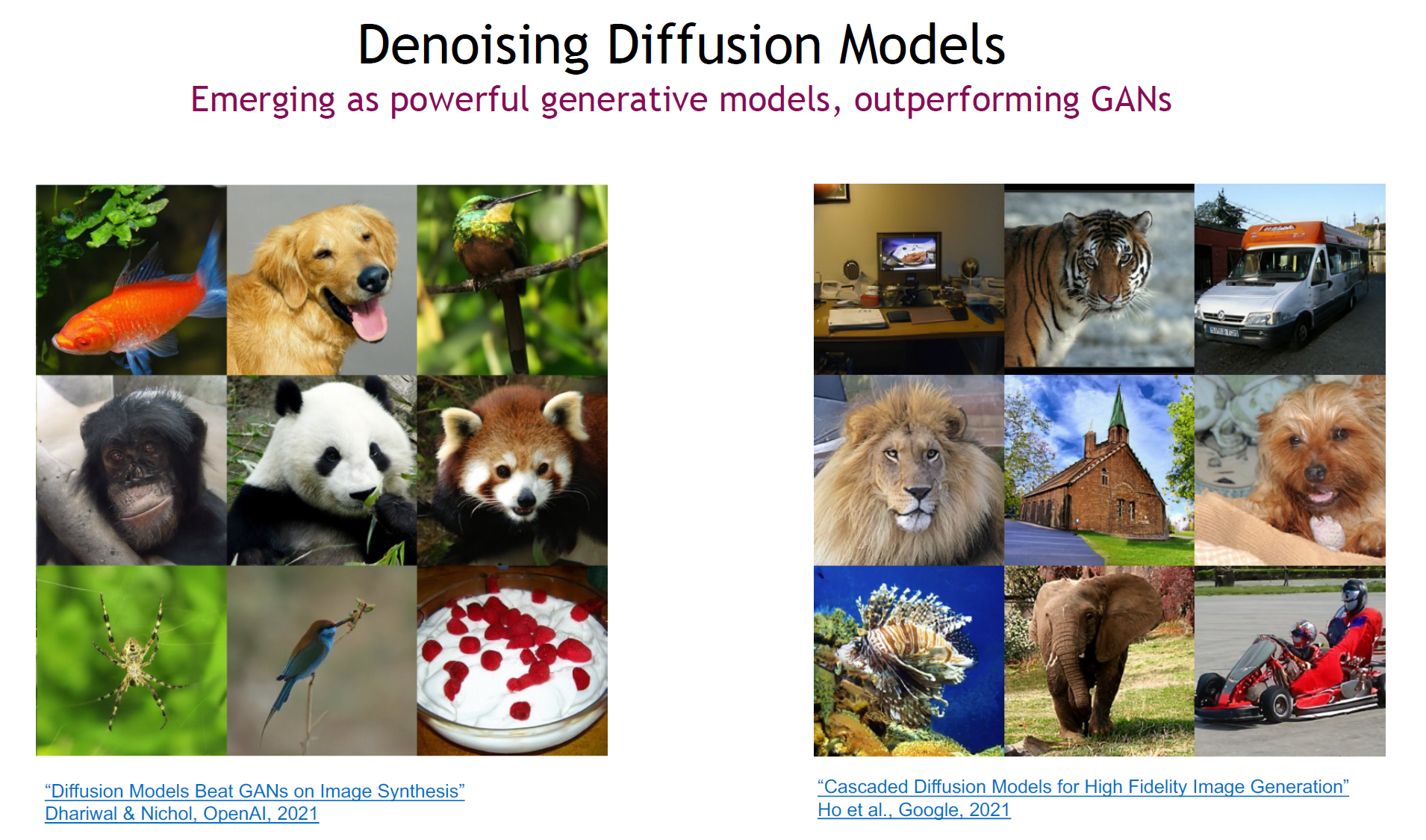
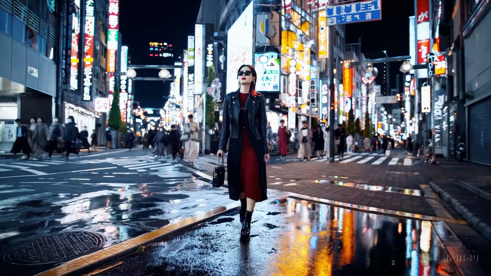
$\color{blue}{\text{Applications - Content Creation outperforming GANs}}$ 
$\color{blue}{\text{Is it possible to implement this model by ourselves?}}$
We are going to implement this generative model step by step tomorrow.
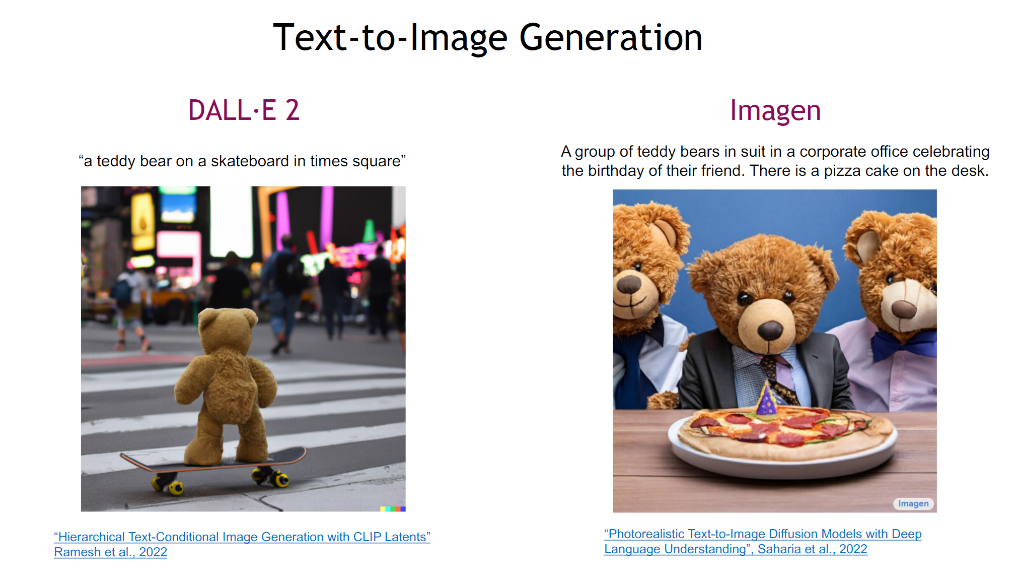
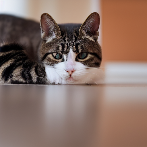
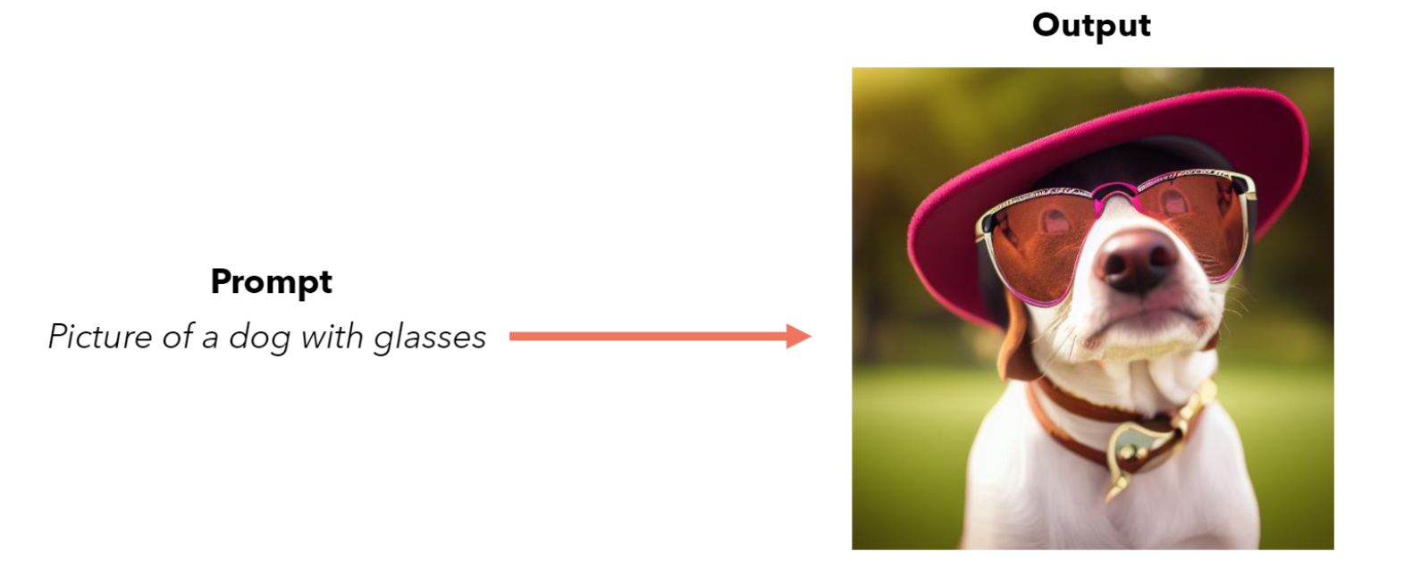
You can write a prompt: $\color{red}{\text{"A cat stretching on the floor, highly detailed, ultra sharp, cinematic, 100mm lens, 8k resolution."}}$
Your model generates:
First, we need to understand the theory.
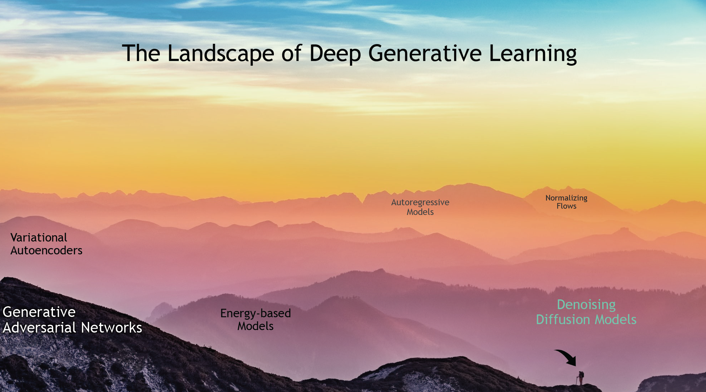
$\color{blue}{\text{Different types of Generative Models:}}$ 
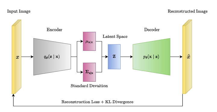
Variational Auto Encoder (VAE)
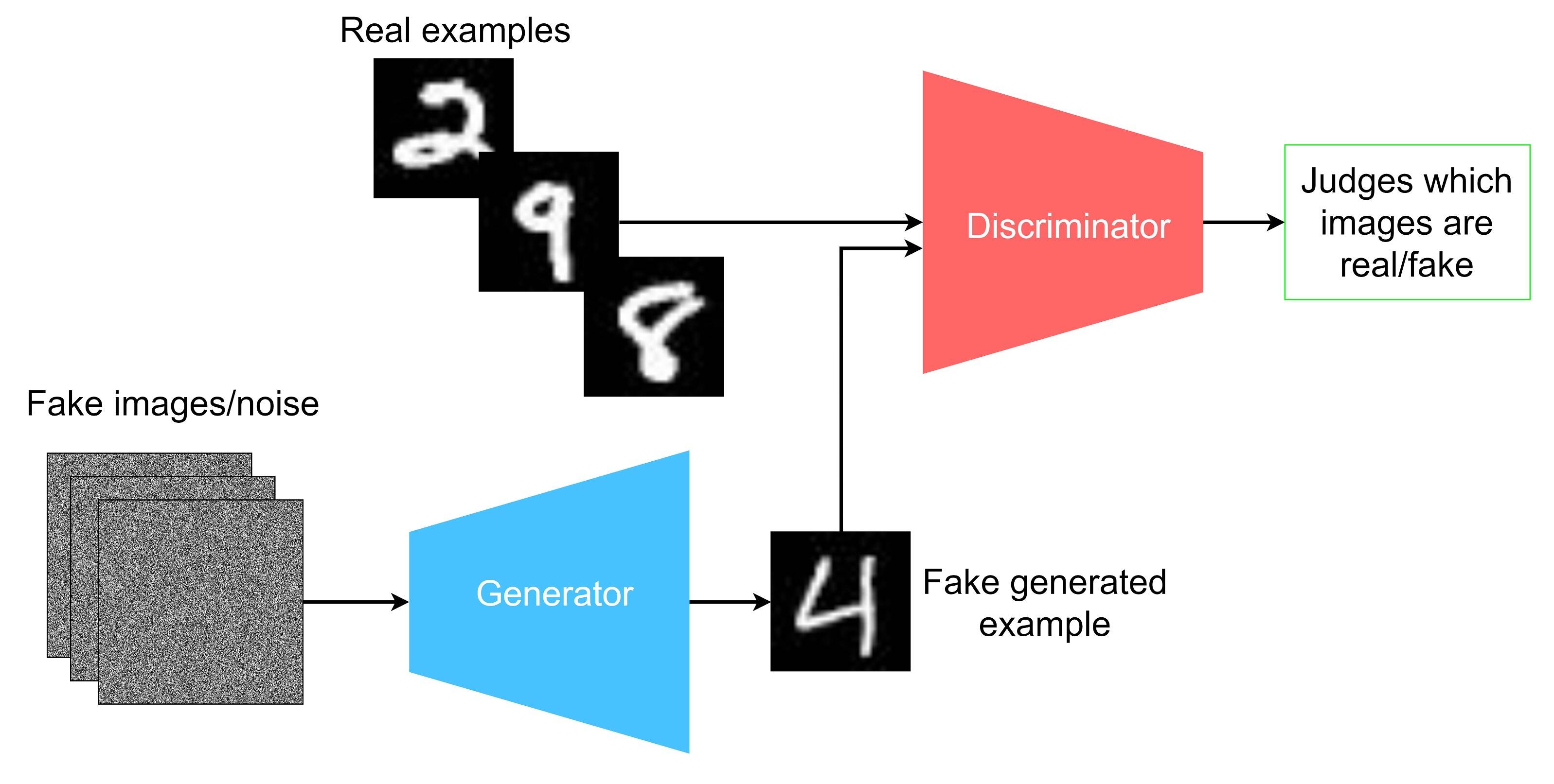
Generative Adversarial Networks(GANs)
Diffusion Models
$\color{blue}{\text{Common Formulation }}$ 
Use a parameterized function to generate data from random noise:
$X = f_{\theta}(z) , \, z\sim \mathbb{N}(0,I) $ (In order to easy generation)
- In VAE the $f_\theta$ is the Decoder function
- In GAN the $f_\theta$ is a Generator function
- How about Diffusion? Add and Remove Noise from the Image
In this talk we find this function for diffusion models
Diffusion function is more complicated than other methods
Lecture Plan
Today's Plan:
- $\color{blue}{\text{Basics of diffusion model}}$
- $\color{blue}{\text{Denoising diffusion models}}$
Tomorrow's Plan:
- $\color{gray}{\text{Conditional diffusion models}}$
- $\color{gray}{\text{Text to image Diffusion Model}}$
- $\color{gray}{\text{Classifier-free Guidance}}$
- $\color{gray}{\text{Latent Diffusion Model (Stable Diffusion Model)}}$
- $\color{gray}{\text{Coding Text to image Diffusion Model from Scratch}}$
$\color{blue}{\text{Basics of diffusion model}}$ 
Start with some questions:
- $\color{red}{Q1}$: Can we have a good characterization of $q(x_1)$??
- $\color{red}{Q2}$: If we have the noise distribution, can we find it?
No because we do not have a good characterization of $q(x_0)$
$\color{blue}{\text{We Need Assumptions}}$ 
What is the noise we add to input?
- We assume $q(x_t|x_{t-1})\sim \mathbb{N}(\sqrt{1-\beta_{t}} \cdot x_{t-1},\beta_t I)$
- We can write it as: $x_t = \sqrt{1-\beta_t}x_{t-1} + \sqrt{\beta_t} \epsilon$ such that $\epsilon \sim \mathbb{N}(0,I)$. Scale down and add noise.
- $0<\beta_i<1$
(Keep this in your memory.)
So Easy!
This is not the only model that you have to use. This is one way to think about it
- Why do we use $\sqrt{1-\beta_{t}}$ and $\sqrt{\beta_t}$ coefficients? Preserving the variance of the data is important because adding noise at certain steps can significantly increase the variance.
- In the forward process, scale down, add a bit of noise, and go to the next step.
$\color{red}{Q1}$: If we start with the input at step zero and want to obtain the noisy image at step 100, how many iterations of the process are required? 100 steps
$\color{red}{Q2}$: Is it possible to directly generate the noisy image at step 100 without using the iterative process?
Let's see what happens:
$x_1 = \sqrt{1-\beta_1} x_0 + \sqrt{\beta_1}\epsilon_0$ such that $\epsilon_0 \in \mathbb{N}(0,I)$
$x_2 = \sqrt{1-\beta_2} x_1 + \sqrt{\beta_2}\epsilon_1$ such that $\epsilon_1 \in \mathbb{N}(0,I)$ Can we combine these two equations?
Replace $x_1$ in second equation:
$x_2 = \sqrt{\underbrace{1-\beta_2}_{\alpha_2}}\sqrt{\underbrace{1-\beta_1}_{\alpha_1}}x_0 + \underbrace{\sqrt{1-\beta_2} \sqrt{\beta_1} \epsilon_0 + \sqrt{\beta_2} \epsilon_1}_{\mathbb{N}(0,[(1-\beta_2)\beta_1 + \beta_2]I)}$
$\color{green}{\text{Definition}}$: $\bar{\alpha_2} = (1-\beta_1)\cdot (1-\beta_2) = \alpha_1 \cdot \alpha_2$
$\mathbb{N}(0,[(1-\beta_2)\beta_1 + \beta_2]I) =\mathbb{N}(0,[\beta_1+\beta_2-\beta_1\beta_2+1-1]) =$
$\mathbb{N}(0,[1-(1-\beta_1)(1-\beta_2)]) = \mathbb{N}(0,[1-\bar{\alpha_2}]) $
Therefore:
$x_2 = \sqrt{\bar{\alpha_2}}x_0 + \sqrt{1-\bar{\alpha_2}}\epsilon$ such that $\epsilon \sim \mathbb{N}(0,I)$ We do not need the iterative process
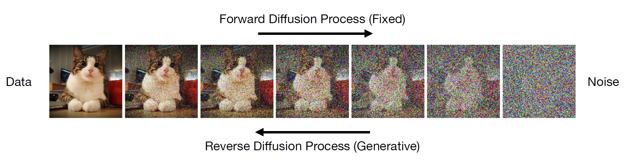
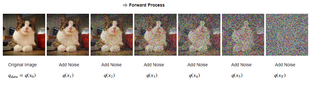
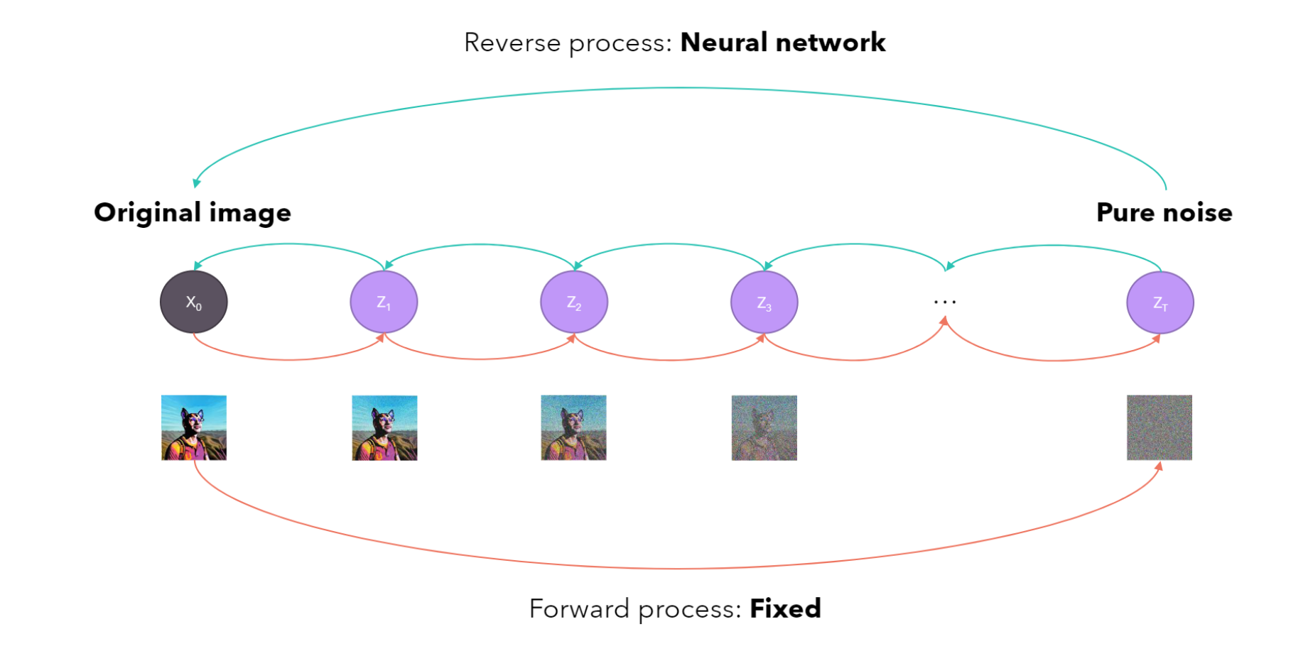
$\color{blue}{\text{Forward Process}}$ 
In general at step $t$ we have:
$x_t = \sqrt{\bar{\alpha_t}}x_0+ \sqrt{1-\bar{\alpha_t}} \epsilon$ such that $\epsilon \sim \mathbb{N}(0,I)$
$\bar{\alpha_t} = \alpha_1 \cdot \alpha_2 \cdots \alpha_t = (1-\beta_1) \cdot (1-\beta_2) \cdots (1-\beta_t)$
$\alpha_i = (1-\beta_i)$
$\color{red}{Q1}$: We take input and add noise, but What? Who cares about it?
$\color{blue}{\text{Let's look at the }\bar{\alpha_t}}$ : 
$\color{red}{Q1}$: What is the range of each $\alpha_i$?? $0<\alpha_i<1$ because $0<\beta_i<1$
We are multiplying $t$ numbers between $0$ and $1$.
$\color{red}{Q2}$: If we assume $\alpha_i=\frac{1}{2} \forall i$ what is the coefficient mulyiply with $x_0$ fot $T=1000$?
- $\bar{\alpha}_{1000} = (\frac{1}{2})^{1000} \rightarrow x_{1000} = \underbrace{(\frac{1}{2})^{500}}_{\frac{1}{2^{500}} \approx 0} x_0 + \sqrt{1-(\frac{1}{2}})^{500} \epsilon$
So in step $1000$ you got noise only. The content is completely destroyed
$\bar{\alpha_t} = 0 $ as $ T \rightarrow \infty \Rightarrow q(x_T|x_0) \rightarrow \mathbb{N}(0,I)$ It does not matter what is the original input.
$\color{blue}{\text{ Why are we adding noise to the input?}}$ 

- Do we have $q(x_0)$? NO
- Do we have $q(x_1)$? NO
...
- Do we have $q(x_T)$? YES $~~~~~~~~~~~$ $q(x_T) \sim \mathbb{N}(0,I)$
$\color{red}{Q1}$: If we have $q(x_{t-1})$, can we have $q(x_t)$??? YES, That is a Forward Process
$q(x_t|x_{t-1}) \sim \mathbb{N}(\sqrt{1-\beta_t} x_{t-1}, \beta_t I)$ or $~~~~~$ $x_t = \sqrt{1-\beta_t}x_{t-1} + \sqrt{\beta_t} \epsilon$ such that $\epsilon \sim \mathbb{N}(0,I)$
$\color{red}{Q2}$: Main Question: Can we come back in this process??
$\color{red}{Q3}$: If we have (assuming) the distribution $q_t$ can we generate the distribution at $q_{t-1}$ ???
$\color{red}{Q4}$: Is it possible $q(x_t) \rightarrow q(x_{t-1})$??
Suppose we can do it. We called this $\color{red}{\text{Reverse Process}}$
$\color{red}{Q5}$: How can we do it???
$\color{blue}{\text{Just we know that $q(x_T)$ is a normal distribution}}$
$\color{blue}{\text{Let's see what is the issue}}$ 
$\color{green}{\text{Our Goal}}$: Find $q(x_{t-1}|x_t)$ (Denoising) If we solve this we done!
One way to simplify this conditional distribution is the Bayse Rule:
$q(x_{t-1}|x_t) = \frac{\overbrace{q(x_t|x_{t-1})}^{\mathbb{N}(\sqrt{1-\beta_t}x_{t-1},\beta_t I)}q(x_{t-1})}{q(x_t)}$
If we start from $x_{1000}$ then we have the $q(x_t)$
How about $q_{x_{t-1}}$? We do not have this term.
$\color{red}{\text{Bayse Rule is not good at all for this!}}$
$\color{blue}{\text{Let's do Maximum Likelihood Estimation}}$ 
$\color{red}{Q1}$: the main question is what is $q(x_{t-1}|x_t)$?? (Denoising) Forget Probability. Think about the denoising process
Do not forget at the end of the day we need to have a generative model
$\color{blue}{\text{Modeling setup:}}$ Model $q(x_{t-1}|x_t)$ with a parametric disribution $P_{\theta}(x_{t-1}|x_t)$
We have a guassian noise at step $1000$ and then we use $P_{\theta}$ model to generate an image at step $999$ (one step back). Continue this process to set $0$
Then we can find the parameters $\theta$ that fit to training samples based on MLE
$\color{red}{Q1}$: what would be a good parametric model (or Distribution)???
We are going to model it as gaussian $\mathbb{N}(\mu_{\theta}(x_t \,\,) , \sigma_t^2I)$
What would be the mean of this Gaussian distribution??? Can be any function?
Should this function be related to step $t$ or not?? Not necessarily but it can be useful.
We can use $\color{blue}{\text{Neural Network }}$(Very good function)
Each time, you cannot find a function with exact math, you can model it with a neural network if you have enough data
$\color{blue}{\text{Model with Neural Network}}$ 
So, we model the distribution as $P_{\theta}(x_{t-1}|x_t) \sim \mathbb{N}(\mu_{\theta}(x_t,t),\sigma_t^2 I)$
Take the input (fully noise), and try to recover the input with lower noise
Given this model we can generate data as:
$P_{\theta}(x_0) = \underbrace{P(x_T)}_{\mathbb{N}(0,I)}P_{\theta}(x_{T-1}|x_T) \cdots P_{\theta}(x_0|x_1)$ This is called $\color{blue}{\text{Diffusion Process }}$.
$\color{blue}{\text{The only Remaining Task is Learning }\theta}$ 
$\color{red}{Q1}$: How to learn $\theta$: parameters of Denoiser to find $\mu_{\theta}(x_t,t)$
What would be the approach: $\color{blue}{\text{Maximum Likelihood Estimation}}$.
$\max_{\theta}\mathbb{E}_{x_0 \sim \underbrace{q(x_0)}_{Real Data}}\big[\log P_{\theta}(x_0)\big] \Rightarrow \theta^*$ we can use it in $\color{blue}{\text{Denoiser}}$
$\color{red}{Q2}$: Can we optimize this Directly?? NO
We need to find a lower bound for likelihood
$\color{blue}{\text{How can we find the lower bound}}$ 
We need to find $q(x_{t-1}|x_t)$ and we model this with $P_{\theta}(x_{t-1}|x_t)=\mathbb{N}(\mu_{\theta}(x_t,t),\sigma_t^2 I)$
KL-Divergence measures the similarity between two distributions
Let's look at: $KL(q||p) = \mathbb{E}_q\big[\log \frac{q}{p}\big]$
$KL\big(q(x_{1:T}|x_0)||P_{\theta}(x_{1:T}|x_0\big)$ The forward process of original distribution and model should be close to each other
$\color{red}{Q1}$: Why do we need to keep conditioning as $q(x_{1:T}|x_0) = q(x_1|x_0) q(x_2|x_1,x_0) \cdots q(x_T|x_{T-1},x_0)$??
$q$ has Markovian property so we can remove $x_0$, but if we remove it from for example $q(x_2|x_1)$ then if we want to compute this, we need to use Bayse rule as $q(x_2|x_1) = \frac{q(x_1|x_2)q(x_2)}{q(x_1)}$ but we do not have $q(x_1)$ and$q(x_2)$
The trick is that to write $q(x_2|x_1) = q(x_2|x_1,x_0) = \frac{q(x_1|x_2,x_0)q(x_2|x_0)}{q(x_1|x_0)}$. Now we have $q(x_2|x_0)$ and $q(x_1|x_0)$
Do not forget that at the end we need to find an approximation of $P_{\theta}(x_0)$ to solve the previous optimization problem
$KL\big(q(x_{1:T}|x_0)||P_{\theta}(x_{1:T}|x_0\big) = \mathbb{E}_{q(x_{1:T}|x_0)}\big[\log \frac{q(x_{1:T}|x_0)}{P_{\theta}(x_{1:T}|\underbrace{x_0}_{\text{We do not want this here}})}\big]$
$ =\mathbb{E}_{q(x_{1:T}|x_0)}\big[\log \frac{q(x_{1:T}|x_0)}{\frac{P_{\theta}(x_{0:T})}{P_{\theta}(x_0)}}\big] = \mathbb{E}_{q(x_{1:T}|x_0)}\big[\log \frac{P_{\theta}(x_0)q(x_{1:T}|x_0)}{P_{\theta}(x_{0:T})}\big] $
$= \mathbb{E}_{q(x_{1:T}|x_0)} \big[\log P_{\theta}(x_0) \big] + \mathbb{E}_{q(x_{1:T}|x_0)} \big[\log \frac{q(x_{1:T}|x_0)}{P_{\theta}(x_{0:T})}\big] $
So we have:
$KL\big(q(x_{1:T}|x_0)||P_{\theta}(x_{1:T}|x_0\big)=$
$\mathbb{E}_{q(x_{1:T}|x_0)} \big[\log P_{\theta}(x_0) \big] + \mathbb{E}_{q(x_{1:T}|x_0)} \big[\log \frac{q(x_{1:T}|x_0)}{P_{\theta}(x_{0:T})}\big] \Rightarrow $
$\mathbb{E}_{q(x_{1:T}|x_0)} \big[\log P_{\theta}(x_0) \big] =$
$\mathbb{E}_{q(x_{1:T}|x_0)} \big[\log \frac{P_{\theta}(x_{0:T})}{q(x_{1:T}|x_0)}\big] + KL\big(q(x_{1:T}|x_0)||P_{\theta}(x_{1:T}|x_0\big) $
$x_0$ is not in $\mathbb{E}_{q(x_{1:T}|x_0)}$ so we have:
$\log P_{\theta}(x_0) = \mathbb{E}_{q(x_{1:T}|x_0)} \big[\log \frac{P_{\theta}(x_{0:T})}{q(x_{1:T}|x_0)}\big] + \underbrace{KL(.||.)}_{\text{Non-negative number}} \Rightarrow$ $\log P_{\theta}(x_0) \ge \mathbb{E}_{q(x_{1:T}|x_0)} \big[\log \frac{P_{\theta}(x_{0:T})}{q(x_{1:T}|x_0)}\big] $
This is the $\color{red}{\text{lower bound}}$
Instead of maximizing $\log P_{\theta}(x_0)$ we have following optimization:
$\max_{\theta }\mathbb{E}_{q(x_{1:T}|x_0)} \big[\log \frac{P_{\theta}(x_{0:T})}{q(x_{1:T}|x_0)}\big] \overbrace{\Rightarrow}^{Add - sign} \min_{\theta} \mathbb{E}_{q(x_{1:T}|x_0)} \big[\log \frac{q(x_{1:T}|x_0)}{P_{\theta}(x_{0:T})}\big]$
Still Difficult
Simplify a bit
$\min_{\theta } - \mathbb{E}_{q(x_{1:T}|x_0)} \big[\log \frac{P_{\theta}(x_{0:T})}{q(x_{1:T}|x_0)}\big] =$
$\min_{\theta } - \mathbb{E}_{q(x_{1:T}|x_0)}\big[\log \frac{P(x_T)\cdot P_{\theta}(X_{T-1}|X_T) \cdots P_{\theta}(X_{0}|X_1) }{q(x_1|x_0) \cdot q(x_2|x_1,x_0) \cdots q(x_T|x_{T-1},x_0)}\big] $
Let's rearrange this term a bit:
$\min_{\theta } - \mathbb{E}_{q(x_{1:T}|x_0)} \big[\log \frac{P(x_T)\cdot P_{\theta}(x_0|x_1) \prod_{t=2}^{T}P_{\theta}(x_{t-1}|x_t)}{q(x_1|x_0) \cdot \prod_{t=2}^{T}q(x_t|x_{t-1},x_0)}\big] = $
$\min_{\theta } - \mathbb{E}_{q(x_{1:T}|x_0)} \big[\log \frac{P(x_T)P_{\theta}(x_0|x_1)}{q(x_1|x_0)} + \sum_{t=2}^{T}\log \frac{P_{\theta}(x_{t-1}|x_t)}{q(x_t|x_{t-1},x_0)}\big]$
$q$ is depended on $x_{t-1}$ and always $x_0$ But $P_{\theta}$ depend on $x_t$
We do not like this and we wish have $q(x_{t-1}|x_t)$ to compare distributions
This is the time to use the Bayse Rule
$q(x_t|x_{t-1},x_0) = \frac{q(x_{t-1}|x_t,x_0) \cdot q(x_t|x_0)}{q_(x_{t-1}|x_0)}$
Replace it
$\min_{\theta } - \mathbb{E}_{q(x_{1:T}|x_0)} \big[\log \frac{\overbrace{P(x_T)}^{\text{Not Depend on} \theta}P_{\theta}(x_0|x_1)}{q(x_1|x_0)} + \sum_{t=2}^{T} \log \frac{P_{\theta}(x_{t-1}|x_t)}{\frac{q(x_{t-1}|x_t,x_0) q(x_{t}|x_0)}{q(x_{t-1}|x_0)}} \big]$
Simplify (given $x_0$ the $q(x_1|x_0)$ is clear and not depend on $\theta$
$\min_{\theta } - \mathbb{E}_{q(x_{1:T}|x_0)} \big[\log \overbrace{P_{\theta}(x_0|x_1)}^{Denoiser \, distribution} \big] -$
$\,\,\,\,\,\,\,\,\,\,\,\,\,\,\,\,\,\,\,\, \mathbb{E}_{q(x_{1:T}|x_0)} \big[\sum_{t=2}^{T}\log \frac{P_{\theta}(x_{t-1}|x_t)}{q(x_{t-1}|x_t,x_0)} + \log \frac{\overbrace{q(x_{t-1}|x_0)}^{Gaussain \, does , depend \, on \, \theta ?}}{\underbrace{q(x_t|x_0)}_{Gaussain \, does , depend \, on \, \theta ?}}\big] $
$\color{blue}{\text{The final loss function is}}$ 
$\min_{\theta}\mathbb{E}_{q(x_t|x_0)}\big[\underbrace{-\log P_{\theta}(x_0|x_1)}_{L_0} + $
$\sum_{t=2}^{T}\underbrace{KL(q(x_{t-1}|x_t,x_0) || P_{\theta}(x_{t-1}|x_t)}_{L_{t-1}} \big]+ Constant$
Let's Look at one of these terms
$\color{red}{\text{What is the intution}}$: We need to find $q(x_{t-1}|x_t)$ but we could not. So we approximate it with $P_{\theta}(x_{t-1}|x_t)$
So one loss function should be the KL-Divergence between them and as you can see we have $KL(q(x_{t-1}|x_t,x_0) || P_{\theta}(x_{t-1}|x_t))$
But we have this $x_0$ in the $q(x_{t-1}|x_t,x_0)$
Math is correct. What is the intuition?? It means that we want to use $P_{\theta}(x_{t-1}|x_t)$ not only do the reverse but also know the $x_0$. We need this direction as a guide because otherwise, we only have noise data.
What is $P_{\theta}(x_{0}|x_1)$?? $\mathbb{N}(\mu_{\theta}(.),\sigma^2I)$
We should quantize this Gaussian distribution to $[0,255]$
$\color{blue}{\text{Is it possible to find an easier way instead of KL}}$: 
$q(x_{t-1}|x_t,x_0) = \frac{\overbrace{q(x_t|x_{t-1},x_0)}^{Gaussain \, Distribution} \cdot \overbrace{q(x_{t-1}|x_0)}^{Gaussain \, Distribution} }{\underbrace{q(x_t|x_0)}_{\mathbb{N}\Big(\sqrt{\bar{\alpha_t}}x_0,(1-\alpha_t)I\Big)}} \Rightarrow$
$q(x_{t-1}|x_t,x_0) \sim \mathbb{N}(\hat{\mu}_t(x_t,x_0),\hat{\beta}_tI)$
such that based on algebraic manipulation
$\hat{\mu_t}(x_t,x_0) = \frac{1}{\sqrt{1-\beta_t}}(x_t - \frac{\beta_t}{\sqrt{1-\bar{\alpha_t}}}\epsilon)$ and $x_t = \sqrt{\bar{\alpha_t}}x_0 + \sqrt{1-\bar{\alpha_t}}\epsilon$ and $\hat{\beta_t} = \frac{1-\bar{\alpha}_{t-1}}{1-\bar{\alpha_t}}\beta_t$
$P_{\theta}(x_{t-1}|x_t) \sim \mathbb{N}(\mu_{\theta}(x_t,t),\sigma^2I)$
So we can compute the KL between two Gaussian distributions in an exact form
$L_0 = P_{\theta}(x_0|x_1) = \mathbb{N}(\mu_{\theta}(x_1,1),\sigma^2I)$ (quantize)
$L_{t-1} =KL(q(x_{t-1}|x_t,x_0) || P_{\theta}(x_{t-1}|x_t) = $
$\mathbb{E}_{q(x_t|x_0)}\Big[\frac{1}{2\sigma_t^2} ||\hat{\mu}_t(x_t,x_0)-\mu_{\theta}(x_t,t)||^2\Big] + Constant $
$\color{blue}{\text{How can we use it for training?}}$ 
- Can we compute $\hat{\mu}_t(x_t,x_0)$ ?
We have $x_0$ try to sample $\epsilon$ from guassian distribution noise and use $x_t$ and compute $\hat{\mu}_t(x_t,x_0)$. It is a fixed vector
- Can we compute $\mu_{\theta}(x_t,t)$?
we have $x_t$ and $t$ already. Then $\mu_{\theta}$ is just a network to map $x_t$ to another vector with the same dimension and try to align it with $\hat{\mu_t}$ by minimizing a quadratic loss
$\color{blue}{\text{Even though It is done, we want to simplify it a bit }}$ 
We can further simplify the objective and training:
- $\hat{\mu_t}(x_t,x_0) = \frac{1}{\sqrt{1-\beta_t}}(x_t - \frac{\beta_t}{\sqrt{1-\bar{\alpha_t}}}\epsilon)$
Reformulate $\mu_{\theta}(x_t,t)$ to be similar to $\hat{\mu}_t(x_t,t)$
- $\mu_{\theta}(x_t,t) := \frac{1}{\sqrt{1-\beta_t}}(x_t -\frac{\beta_t}{\sqrt{1-\bar{\alpha_t}}}\underbrace{\epsilon_{\theta}(x_t,t)}_{Neural Network}) $
$L_{t-1}= \mathbb{E}_{q(x_t|x_0)}\Big[\frac{1}{2\sigma_t^2}||\frac{1}{\sqrt{1-\beta_t}}x_t - \frac{\beta_t}{\sqrt{1-\beta_t}\sqrt{1-\bar{\alpha_t}}}\epsilon - \frac{1}{\sqrt{1-\beta_t}}x_t + $
$\frac{1}{\sqrt{1-\beta_t}}\frac{\beta_t}{\sqrt{1-\bar{\alpha_t}}}\epsilon_{\theta}(x_t,t)||^2\Big]$
$L_{t-1} = \mathbb{E}_{q(x_t|x_0)}\Big[\underbrace{\frac{1}{2\sigma_t^2}\frac{\beta_t^2}{(1-\beta_t)(1-\bar{\alpha_t})}}_{Constant}||\epsilon - \epsilon_{\theta}(x_t,t)||^2\Big]$
The whole optimization is
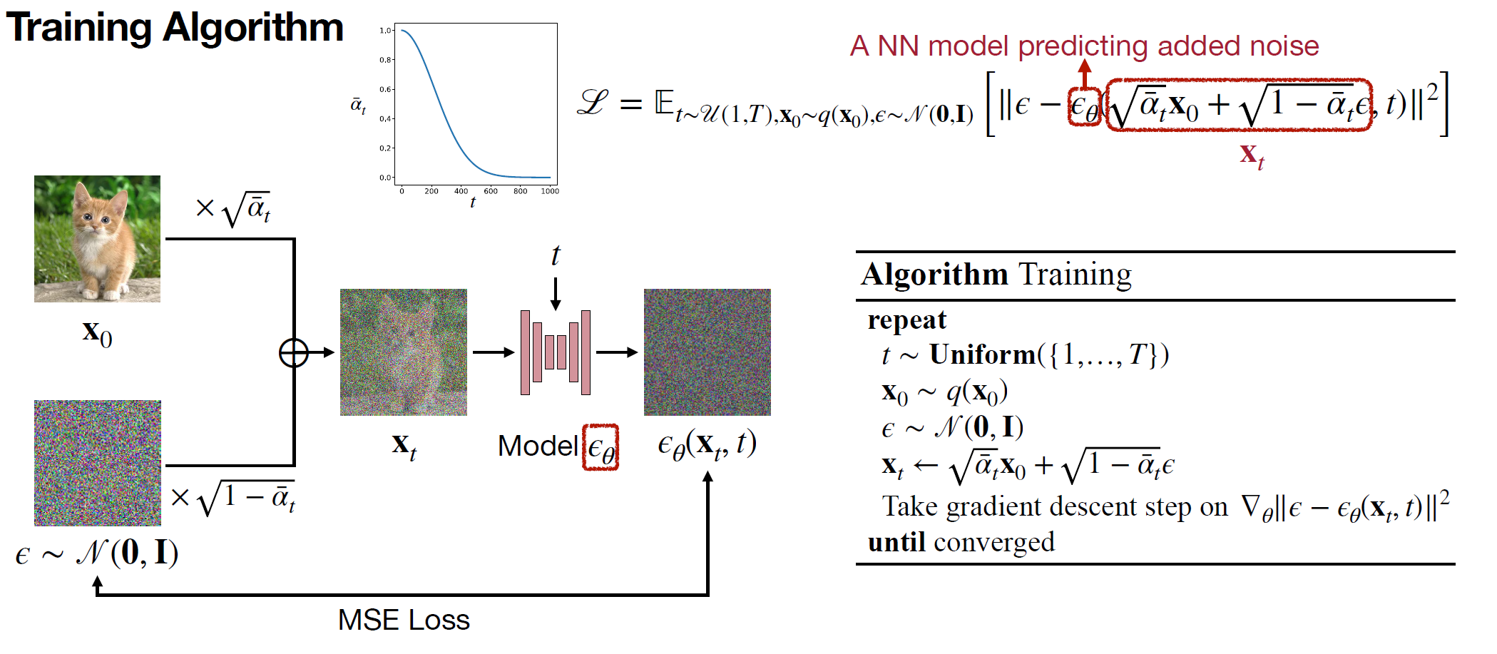
$\min_{\theta} \mathbb{E}_{q(x_t|x_0)} \big[\lambda_t ||\epsilon - \epsilon_{\theta}(x_t,t)||^2\big]$
$\color{blue}{\text{training process }}$ 
- get sample $\epsilon \sim \mathbb{N}(0,I)$ and $t\sim Uniform(0,I)$
- we can compute $x_t$ by $q(x_t|x_0)$ (ADD NOISE)
- Learn $\theta$, parameter vectors of the reverse process (NN model). When we learn $\theta$, we have $P_{\theta}(x_{t-1}|x_t) \sim \mathbb{N}(\mu_{\theta}(x_t,t),\sigma^2_tI)$
- The only thing that remain is $\lambda_t$ constant that we can compute based on $\beta$.
Is it possible to consider $\lambda_t = 1$?? Yes, and empirically they showed that it works better.
So in the training phase, we minimize the following loss function:
$\mathbb{E}_{\epsilon \sim \mathbb{N}(0,I),q(x_0),t \sim uni(0,T)}\Big[||\epsilon - \epsilon_{\theta}(x_t,t)||^2\Big]$
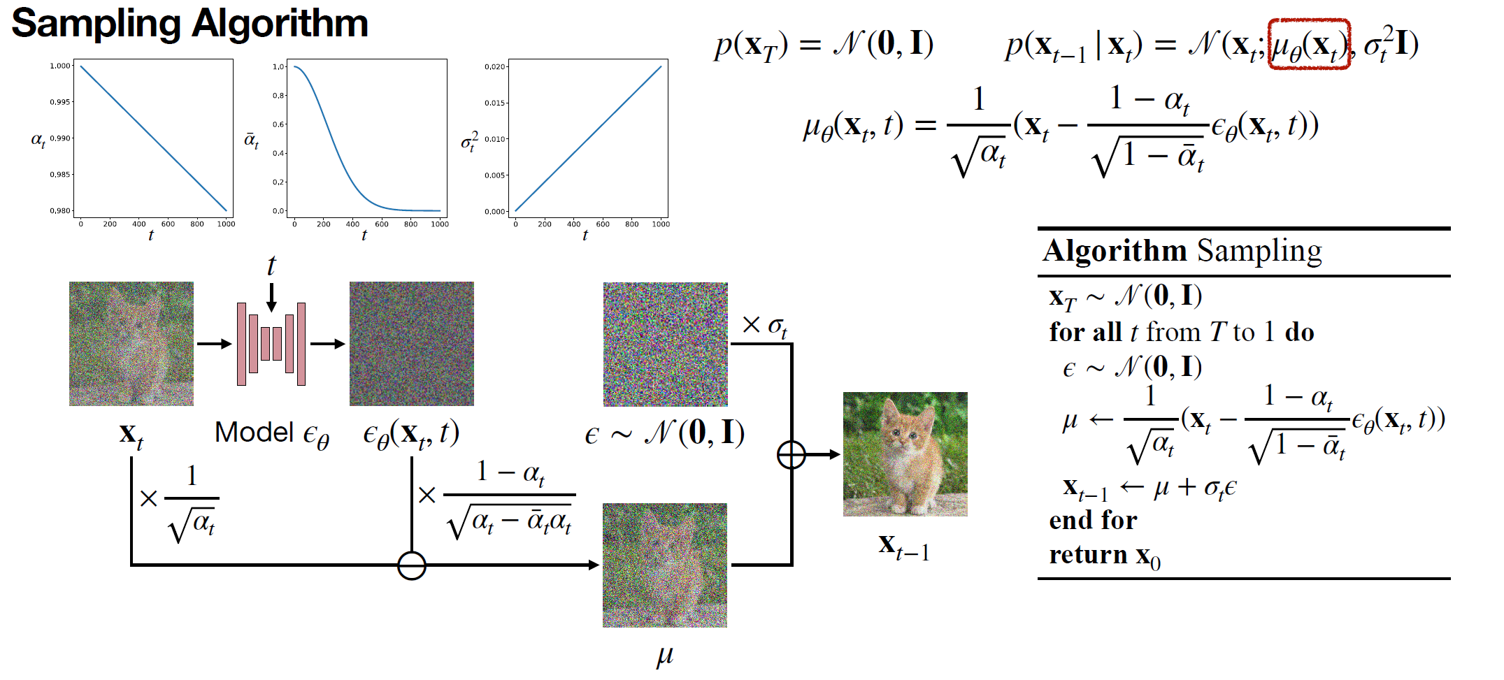
$\color{blue}{\text{Inference time }}$ 
In the inference time we have $\theta^* \Rightarrow \mu_{\theta^*}(x_t,t) \Rightarrow P_{\theta}(x_{t-1}|x_t) \sim \mathbb{N}(\mu_{\theta^*}(x_t,t),\sigma_t^2I)$
They called this process: $\color{red}{\text{Denoising Diffusion Probability Model }}$
There are many variations based on this method
$\color{blue}{\text{Interpretation of Diffusion models with "Score function" }}$ 
We can Imagine that we have the true density function for input $q_{True}(x)$ (we do not have it suppose we have)
The score function is defined as : $S(x) = \nabla_x \log q(x)$
$S(x)$ is a vector with same size as $x$
If we replace the $q(x)$ with $q_{True}(x)$ then we can compute $ S^*(x)$
$\color{red}{Q1}$: What would happen if we start from point $x$ and go through the score : $x + \underbrace{\delta}_{Scale}S^*(x) \rightarrow x^\prime$?
This is a step gradient ascent and we can provide a point with a higher likelihood
$\color{red}{\text{IDEA}}$: IF we have $S^*(x)$, can we start from a random point and apply the score function repeatedly?
Let start with Gaussain Distribution:$\mathbb{N}(0,I)$
$x^{(k+\delta)} \leftarrow x^{(k)} + \delta S^*(x^{(k)})$ change the distribution at each step
$\color{red}{Q1}$: Would the end distribution converge to True distribution $q_{True}$?
Each point that changes reaches the local maximum so we converged to some local maximum points
Theorem: By adding a tiny noise to each step we will converge to $q_{True}$
$x^{(k+\delta)} \leftarrow x^{(k)} + \delta S^*(x^{(k)}) + \sqrt{2\delta}\epsilon$ such that $\epsilon\sim \mathbb{N}(0,I) \Rightarrow Dist(x^{(\infty)})= q_{True}$
This is based on the Langevin equation + Brownian motion ( skip the proof)
So, If we have score for True distribution ($\nabla_x \log q_{True}(x)$) then we have a way to generate sample and this is look like to reverse process of Diffusion
We have a generative model $\Rightarrow$ start with a normal distribution $\Rightarrow$ follow the score direction + noise $\Rightarrow$ Finally we have $q_{True}$
But the main problem is that we do not have $q_{True}$ and score function (If we have $q_{True}$ we can sample from it and do not need this process
Q: Can we estimate the ground truth score $S^*(x)$ using a neural network?
We need to find $S_{\theta}(x) \approx S^*(x)$ Can we do it?
Provide a loss function as:
$\min_{\theta} \mathbb{E}_{x\sim q_0(x)}\big[||S_{\theta}(x) - S^*(x)||^2 \big] \Rightarrow$
$\min_{\theta} \mathbb{E}_{x\sim q_0(x)}\big[Tr(\overbrace{\nabla_xS_{\theta}(x)}^{Hessian}) + \frac{1}{2} ||S_{\theta}||^2 \big] $ (Implicit Score Matching) (Computationally Expensive)
Simplify the optimization
$\hat{x} = x + \sigma \epsilon$ such that $\epsilon \sim \mathbb{N}(0,I)$
$\min_{\theta} \mathbb{E}_{q(x,\hat{x})}\Big[\frac{1}{2} ||S_{\theta}(\hat{x}) - \underbrace{\nabla_{\hat{x}}\log q_{\sigma}(\hat{x}|x)||^2}_{\text{Score for Gaussian Density}}\Big]$
Side Note (Score for Gaussian Density)
**if $q \sim \mathbb{N}(0,I)$ then $S(x) = \nabla_x \log C e^{-\frac{||x||^2}{2}} = \nabla_x \big(\frac{-||x||^2}{2}\big) = -x$ **
So we have:
$\nabla_{\hat{x}}\log q_{\sigma}(\hat{x}|x)||^2 = \frac{1}{\sigma^2}(x-\hat{x})$
Therefore
$\min_{\theta} \mathbb{E}_{x \sim q_0(x) , \epsilon \sim \mathbb{N}(0,I)}\Big[\frac{1}{2}||\sigma^2S_{\theta}(\hat{x}) - (\underbrace{x-\hat{x})}_{\epsilon}||^2\Big]$
Compare it with DDPM objective
$\min_{\theta} \mathbb{E}_{x\sim q_0(x) , \epsilon \sim \mathbb{N}(0,I), t \sim uni(0,T)} \Big[||\epsilon_{\theta}(\hat{x},t) - \epsilon||^2\Big]$
The same objective with different interpretation
In score matching, we can say denoising means going in the direction of the maximum log-likelihood and this is called Denoising score matching
$\color{red}{\text{Move to Computer Engineering }}$ 
Denoising Diffusion Probabilistic Models (DDPM)
Denoising Diffusion Probabilistic Models (DDPM)
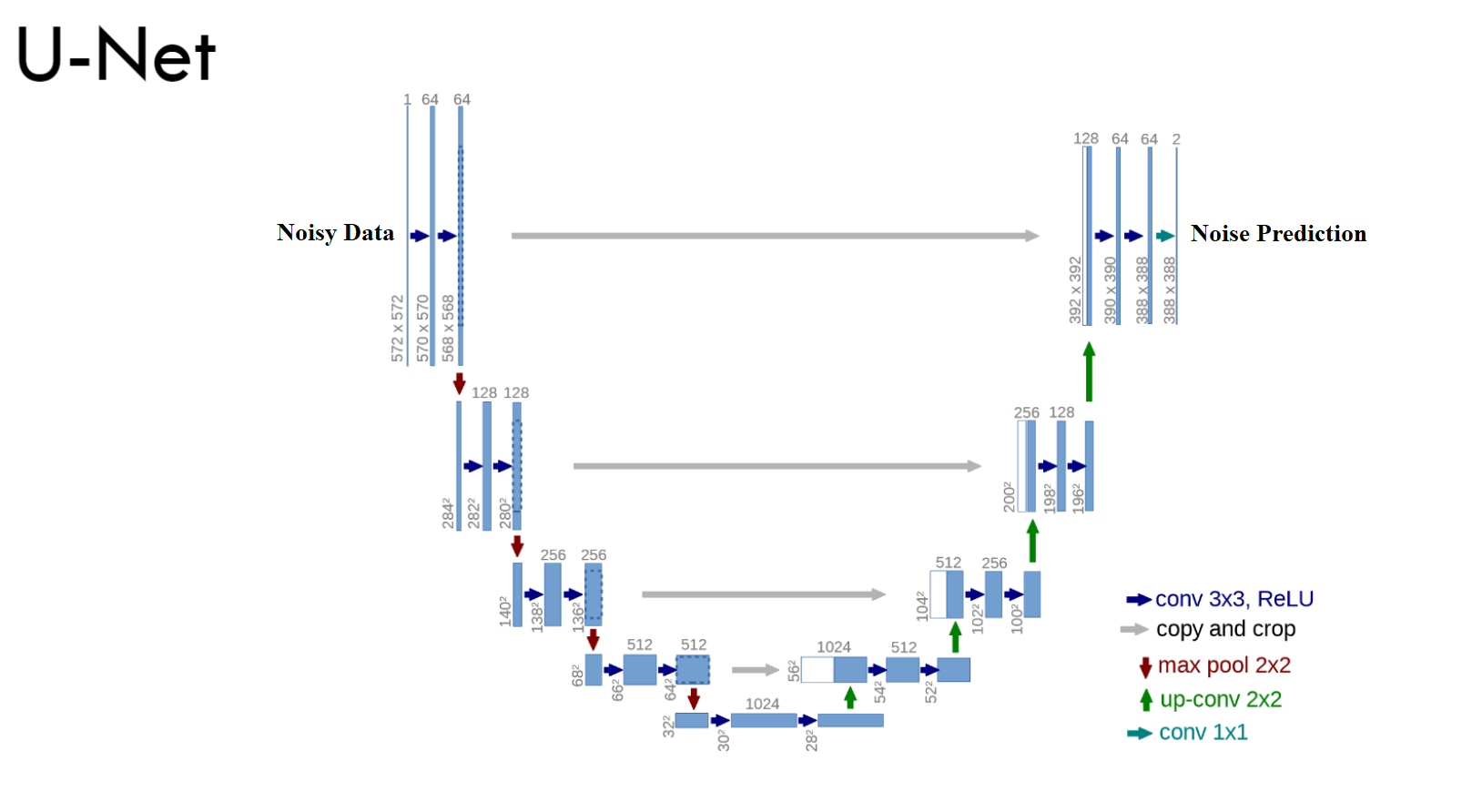
$\color{blue}{\text{What is the Model we use for prediction}}$ 
Lecture Plan
Today's Plan:
- $\color{gray}{\text{Basics of diffusion model}}$
- $\color{gray}{\text{Denoising diffusion models}}$
Tomorrow's Plan:
- $\color{blue}{\text{Conditional diffusion models}}$
- $\color{blue}{\text{Text to image Diffusion Model}}$
- $\color{red}{\text{Classifier-free Guidance}}$
- $\color{red}{\text{Latent Diffusion Model (Stable Diffusion Model)}}$
- $\color{blue}{\text{Coding Text to image Diffusion Model from Scratch}}$
$\color{blue}{\text{Final Goal of Today}}$ 
$\color{blue}{\text{Review From Yesterday}}$ 
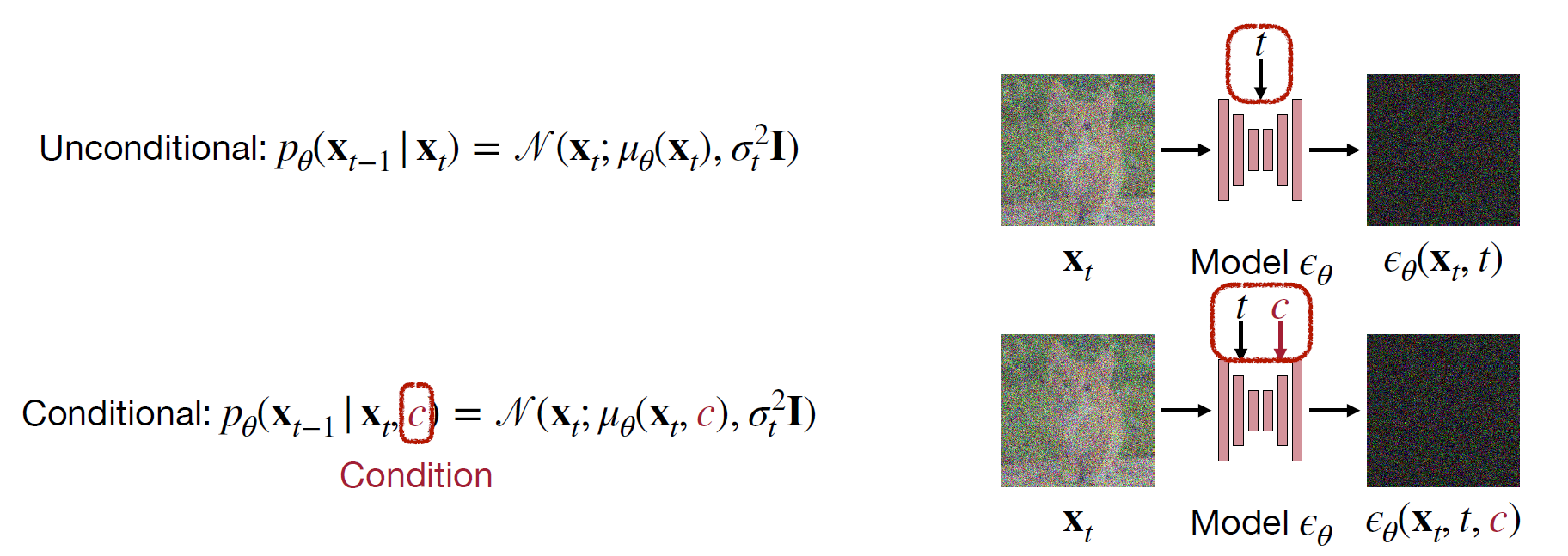
$\color{blue}{\text{Unconditional Models v.s. Conditional Models }}$ 
Condition Types
- Scalar condition: condition on a single scalar (e.g., class ID “cat”)
- Text condition: condition on a sequence of text tokens (e.g., “photo of a moon gate”)
- Pixel-wise condition: condition on a spatial map (e.g., semantic map, canny edge)
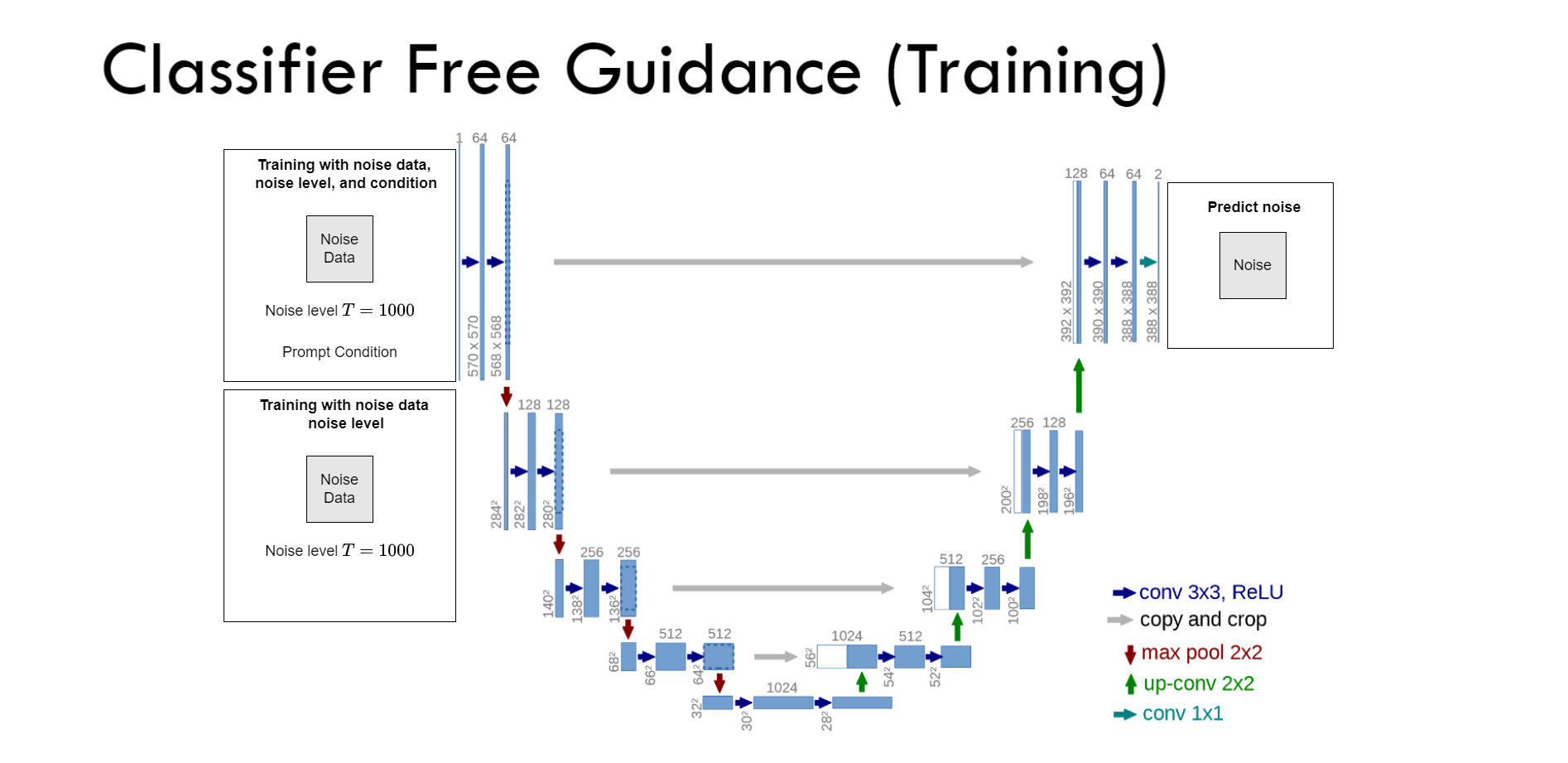
$\color{blue}{\text{Classifier-free Guidance (Training)}}$ 
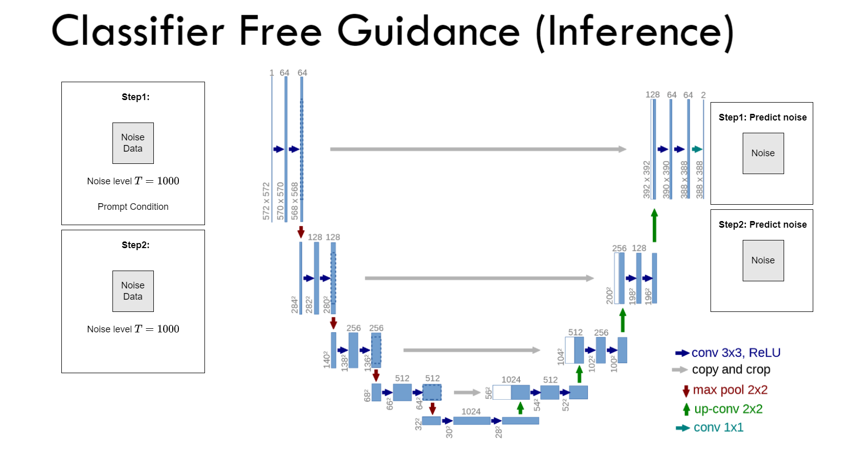
$\color{blue}{\text{Classifier-free Guidance (Inference)}}$ 
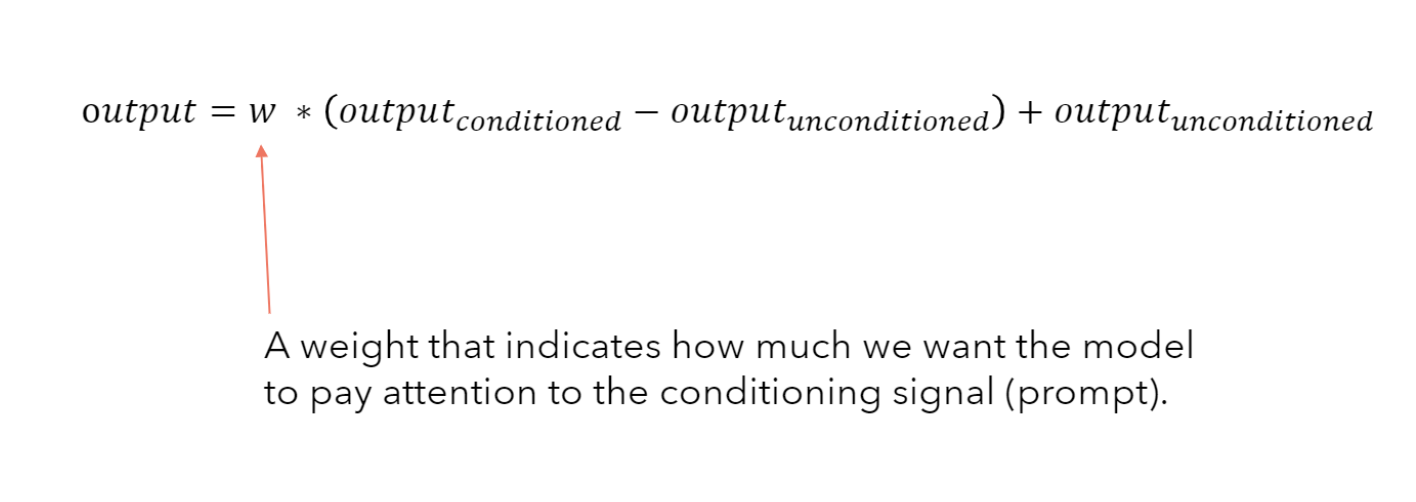
$\color{blue}{\text{How can we combine them}}$ 
$\color{blue}{\text{How can we Encode The text in the prompt}}$ 
Clip: Contrastive Language-Image Pretraining (developed by OpenAI in 2021) 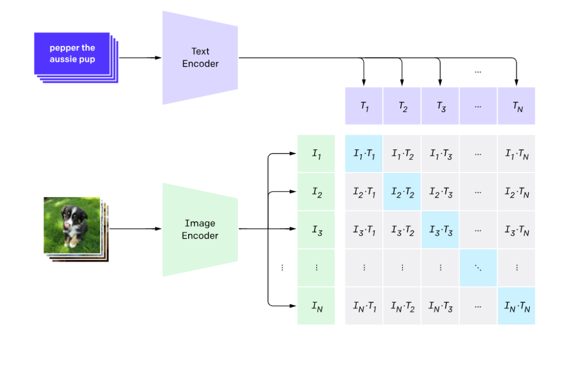
$\color{blue}{\text{Latent Diffusion Model}}$ 
Images are high-resolution data and in DDPM we need to work with a huge vector (for example 1024*1024) What is the solution? Use Encoder-Decoder to compress the input to latent space, then do the diffusion process on latent space and encode it.
What type of Encoder-decoder architecture do we have in the Machine learning Domain?
- AutoEncoder
The code learned by AutoEncoder does not have any semantic meaning
- Varational AutoEncoder Instead of learning a code, Learn a latent Space ( multivariate Normal Distribution)
$\color{blue}{\text{We can Combine ALL}}$ 
$\color{blue}{\text{We can Combine ALL}}$ 
$\color{red}{\text{Move to Implementation }}$ 
Go through the code step by step
- Download the zip file, extract it in your Google Drive, and open Stablediffusion.ipynb in "sd" directory
$\color{blue}{\text{Evaluation For credit}}$
Write a short report to answer the following questions and send it to my email address: $\color{blue}{\text{seyedhamidreza.mousavi@mdu.se}}$
- Run the code with "do_cfg= True" and "do_cfg =False" and use the same prompt and seed and send the results
- Try to edit an image by using the same prompt and changing the "strength" parameter (4 different values) and send the results
- Compare the inference time for running on T4 GPU (Colab default GPU) and Colab CPU. report the time of inference (you can use the time library in Python to compute inference time)
$\color{blue}{\text{Refrences}}$
- Ho, Jonathan, Ajay Jain, and Pieter Abbeel."Denoising diffusion probabilistic models", Conference on Neural Information Processing Systems (NeurIPS 2020)
- Rombach, Robin, et al. "High-resolution image synthesis with latent diffusion models." Proceedings of the IEEE/CVF conference on computer vision and pattern recognition (CVPR). 2022.
- Radford, Alec, et al. "Learning transferable visual models from natural language supervision." International conference on machine learning. PMLR, 2021.
- Ho, Jonathan, and Tim Salimans. "Classifier-free diffusion guidance." arXiv preprint arXiv:2207.12598 (2022).